Parallel Merge Sort Algorithm
Introduction
A sorting algorithm is used to arrange elements of a list/array in a specific order (ascending or descending). For example,

Here, we are sorting the array in ascending order.
This procedure can be finished using a variety of sorting methods. And depending on the needs, we may utilise any algorithm. Different Sorting Algorithms are:
- Bubble Sort
- Selection Sort
- Insertion Sort
- Merge Sort
- Quicksort
- Counting Sort
The time complexity and space complexity of the algorithm impact the efficiency of any sorting algorithm.
- Time Complexity: In relation to the amount of the input, time complexity describes how long it takes an algorithm to execute. It can be shown in a variety of ways:
- Big-O notation (O)
- Omega notation (Ω)
- Theta notation (Θ)
2. Space Complexity: The term “space complexity” refers to how much memory the method need to run completely. Both the input and the auxiliary memory are included.
The additional memory that the algorithm uses in addition to the input data is known as the auxiliary memory. Usually, while calculating an algorithm’s space complexity, auxiliary memory is taken into account.
In this blog, we will discuss in detail merge sort, with special emphasis to parallel merge sort.
Sorting in parallel:
Why do we need parallel sorting?
The process of sorting a list of elements is fairly frequent. When we need to sort a sizable amount of data, a sequential sorting method could not be effective enough. Therefore, parallel algorithms are used in sorting.
What is the potential speed-up with parallel sorting?
If we talk about sequential sorting, its best complexity turns out to be O(nlogn). Using parallel sorting, if we have n processors, its optimal complexity turns out to be O(nlogn)/n = O(log n).
Merge sort
Merge sort is a popular and efficient sorting algorithm that uses a divide-and-conquer approach to sort a list of items. The algorithm works by dividing the input list into two smaller sublists, sorting each of the sublists, and then merging the two sorted sublists back together to form the final sorted list. Additionally, because the algorithm uses a recursive approach, it is relatively simple to implement and understand. Overall, merge sort is a powerful and efficient sorting algorithm that is well-suited for many different applications.
Here is an example of how merge sort works:
Suppose we have the following list of numbers that we want to sort: [6,35,42,15,3,17,63,12]. We can use merge sort to sort this list as follows:
1. Divide the input list into two smaller sublists: [6,35,42,15] and [3,17,63,12].
2. Sort each of the sublists using merge sort: [6,15,35,42] and [3,12,17,63].
3. Merge the two sorted sublists to produce the final sorted list: [3,6,12,15,17,35,42,63].
Time and space complexity:
The time complexity of merge sort is O(n log n) in the average and worst-case scenarios. This means that the algorithm is able to sort large lists of items very quickly, making it a popular choice for many applications.
In terms of space complexity, merge sort has a space complexity of O(n) in the average and worst-case scenarios. This means that the algorithm requires a relatively large amount of memory to sort a list of items. However, because the algorithm uses a recursive approach, the memory requirements can be managed by using an in-place implementation of the algorithm, which can reduce the space complexity to O(1) in the best-case scenario.
Pseudo Code:
function mergeSort(list):
// Check if the list has only one element
if list.length == 1:
return list
// Divide the list into two equal-sized sublists
left = list[:list.length / 2]
right = list[list.length / 2:]
// Sort the left and right sublists
left = mergeSort(left)
right = mergeSort(right)
// Merge the two sorted sublists into a single sorted list
return merge(left, right)
function merge(left, right):
result = []
// Compare the elements from the left and right sublists
// and add the smaller element to the result list
while left.length > 0 and right.length > 0:
if left[0] < right[0]:
result.append(left[0])
left.pop(0)
else:
result.append(right[0])
right.pop(0)
// Add the remaining elements from the left sublist to the result list
while left.length > 0:
result.append(left[0])
left.pop(0)
// Add the remaining elements from the right sublist to the result list
while right.length > 0:
result.append(right[0])
right.pop(0)
return result
This is just one possible way that merge sort can be used to sort a list of numbers. There are many other variations of the algorithm that use different approaches to dividing and merging the sublists. However, the basic idea is always the same: divide the input list into smaller sublists, sort the sublists, and then merge the sorted sublists to produce the final sorted list.
Parallel Merge Sort:
Let’s say we want to rework merge sort so that it can operate on a parallel computing environment. It will be easier for us to develop a parallel merge sort algorithm if we first think about how it would work on an abstract PRAM machine, much as it is advantageous for us to abstract away the specifics of a certain programming language and use pseudocode to explain an algorithm.
Parallel merge sort is a variation of the merge sort algorithm that takes advantage of parallel computing to sort large datasets more quickly. In a parallel merge sort, the initial list is divided into smaller sublists, which are then sorted using multiple CPU cores or processing units simultaneously. This allows the sorting process to be completed more quickly, reducing the overall time complexity of the algorithm.
Finding the actions that might be performed concurrently is the key to constructing parallel algorithms. This occasionally entails examining a well-known sequential method to search for potential simultaneous operations.

Case 1: Fine-grained parallel merge sort
Consider a PRAM machine that has n processors. Though improbable in reality, n >= N, the size of our data to be sorted, might be a theoretically feasible situation if we had a lot of processors. Fine-grained parallelism is the term used to describe this mostly unworkable condition. The fine-grained example is a valuable starting point for ultimately arriving to course-grained solutions, but we’ll look at the more relevant course-grained situation (n<< N) later.
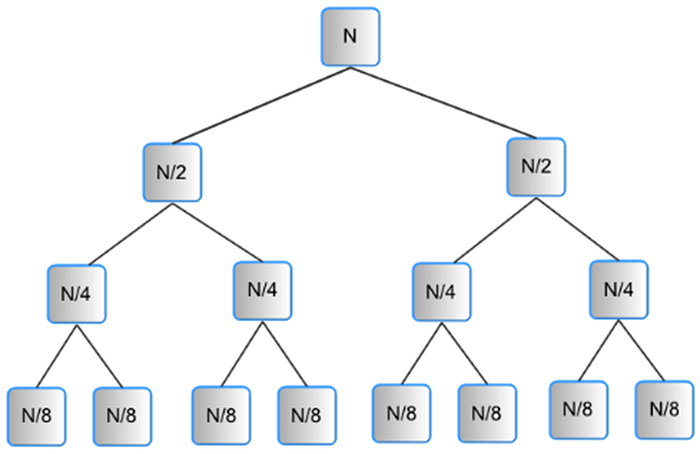
Let’s attempt examining the original method to see where we can run many operations at once. Looking at the recursion tree of the sequential merge sort algorithm can help you understand what is going on and analyse the complexity of the method. Following figure shows the recursive calls to the mergeSort() function as boxes, with the number of items each recursive call would be working on.

Let’s now look at whether of these procedures, which were performed sequentially, may be performed concurrently on different processors. Doing the work necessary at each level of the tree in the above figure concurrently is a logical approach to divide the work that may be executed “in parallel.” Be aware that while thinking about a parallel solution, we employ an iterative strategy and picture starting our work at the bottom of the tree and working our way up one level at a time. Simply put, each process is doing a merging on a subset of the array’s contents.
Following figure shows an example of 8 elements to be sorted and what would result at each level of the tree. Since there is no actual labour at the level of a tree’s leaves, we may start by seeing that level as the N data items that our processors share in memory. At the following level, each of four processors can operate on separate groups of two different data items and combine them. Once those are finished, two processors may each begin working on merging to produce a list of four sorted things. After that, a third processor can combine those two lists of four to get the ultimate list of eight sorted items. This becomes our parallel merge sort algorithm.

Pseudo Code:
procedureparallelmergesort(id, n, data, newdata)
begin
data = sequentialmergesort(data)
for dim = 1 to n
data = parallelmerge(id, dim, data)
endfor
newdata = data
end
Time and space complexity:
In parallel merge sort algorithm, we have n processors. Logn time is required to divide it, and logn time to merge it. So in total, 2logn i.e. O(Logn) is the time complexity for this algorithm. O(n) is the space complexity for parallel merge sort.
Case 2 : a scalable version of parallel merge sort
We probably wouldn’t have enough processors to perform the preceding technique efficiently for big quantities of N. The benchmark is to run these sorting algorithms with extremely high amounts of data items to measure how well the machine works. Sorting is sometimes conducted as a “benchmark test” on very large parallel clusters, although even then, the number of processors is fewer than the number of data items. However, the prior algorithm enables us to comprehend the potential advancement that may be produced when using several processors to address the issue. Let’s move on to an example that is more realistic.
As we’ve already established, the most likely scenario is one in which there are far fewer processors than components that need to be sorted. In this situation, we need a plan for dividing the work that has to be completed on each available processor. We may get started by deciding on a fair number of processors that are readily available. On multicore computers, the operating system may inform us when we begin the sort; in other words, we would request a set of processors from the OS.
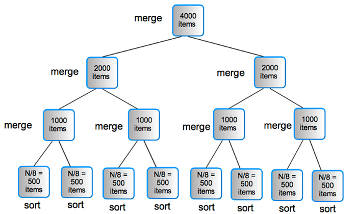
Still, it is feasible to think of utilising a binary tree as an example of the technique. We begin by setting the number of leaf nodes of the tree to n given the number of processors to be used, n. Although it makes the method more understandable to think about n as a power of 2, different values of n are compatible with the procedure. First, each of the n nodes sorts N/n of the original input data values using a quicksort-style rapid sequential sort mechanism. A “parent” process may then be used to combine two sorted lists. Another parent process may utilise the freshly sorted list and combine it with a second child-sorted list.

That was all about parallel merge sort algorithm. Thank you!
